Introduction
Tutorials
Getting familiar with GeoData Manager
Changing how GeoData Manager looks
Scenarios for using GeoData Manager
Data types and nodes
Help with data types and nodes
Getting familiar with GeoData Manager
Changing how GeoData Manager looks
Scenarios for using GeoData Manager
Help with data types and nodes
This tutorial creates a contour map in Surfer of the temperature at -500 m elevation, from the sample database, for example for a report.
We will create four files for Surfer:
A file of temperature in selected wells at -500 m elevation. This has two purposes, to provide the grid for creating the contour map, and to allow us to mark the position of each well trace at -500 m.
A file of wellhead coordinates, to allow us to mark the location of each wellhead on the map.
A file of well traces, to allow us to display these on the map.
A file of well bottomhole coordinates. We want to label each well with the well's name, and if we label the wellheads then the labels at each drilling pad will usually overlap. So, we use this file so we can label the bottom of each well instead, which do not tend to overlap.
Create the file of temperature at -500 m elevation first in case there is a problem, for example not enough data at this elevation.
You will also need a geo-referenced topographical map for Surfer's base map.
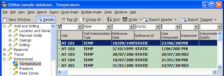
We assume that the most reliable measures of temperatures down the well are the interpreted temperatures, so we will use these temperatures. In the sample database, go to the node Interpreted: Temperature.
In the filter bar, click  and click
 Default Filter in case the filter was different.
Select temperature data sets of type STATIC: In the filter bar, click the  to the right of Reference ID and click
 STATIC in the list.
Click Tag All:
You should now check that there are enough wells to make the final map worthwhile; here there are enough.
Click Map:
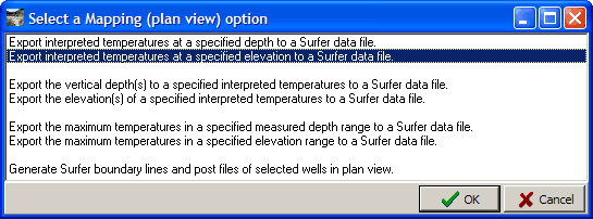
Click Export interpreted temperatures at a specified elevation ... and click OK. Now answer some questions ...
Interpretations below wellbottom ? (optional):
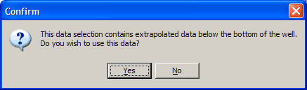
Geodata Manager asks this if one or more tagged wells have interpreted temperatures extrapolated to depths below the bottom of the well:
Click Yes if you are confident in these extrapolations, and GeoData Manager will use these extrapolations if necessary (ie if the elevation of interest is below the bottom of the well and is above the deepest interpreted temperature).
Otherwise click No and GeoData Manager will not use these extrapolations.
In this tutorial, click Yes.
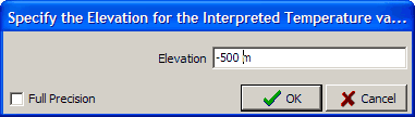
Enter the elevation for the temperatures and click OK:
Elevation above interpretations ?:
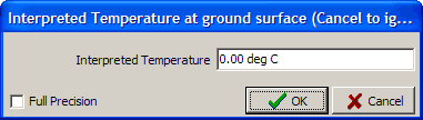
Temperature interpretations typically do not extend up to ground level. If your elevation of interest is close to ground level, then it may be above any interpreted temperatures in one or more wells. You can:
Enter a temperature at ground level (say 20 C) and click OK: GeoData Manager will use all tagged wells, and if necessary extrapolate interpreted temperatures up to the elevation of interest.
Otherwise do not enter a temperature and click Cancel: GeoData Manager will ignore wells where the shallowest interpreted temperature is below the elevation of interest.
In this case the elevation is well down the wells, so it does not matter which you do.
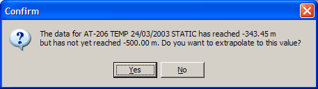
Extrapolate down ?:
For each well whose deepest interpreted temperature is above the elevation of interest, Geodata Manager asks if you want it to extrapolate down to calculate a temperature at the elevation of interest.
If the deepest interpreted temperature is well above the elevation of interest, click No, as in this case:
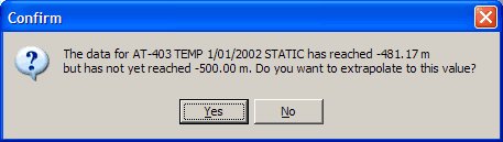
If the deepest interpreted temperature is not far above the elevation of interest, click Yes, as in this case:
If you have clicked No to many wells, you should now ensure that there are enough wells to make the final map worthwhile; here there are enough.
The result is a csv file: select a folder and file name and click OK. Here is the file, opened in a spreadsheet:
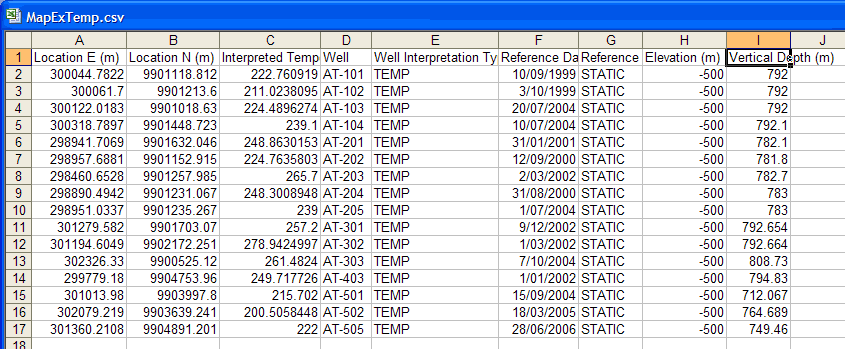
Note Geodata Manager usually makes two interpolations here, which are usually well-behaved:
It is unlikely that the well deviation has been measured at the elevation of interest (unless it is a vertical well), and so Geodata Manager interpolates the well deviations to find the location E and N of the well at the elevation of interest.
It is unlikely that the well temperature has been interpreted at the elevation of interest, and so Geodata Manager interpolates the well temperatures to find the temperature at the elevation of interest.
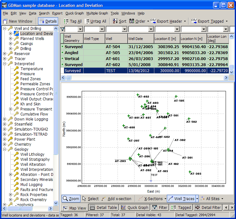
Now, we will tag the wells to appear on the surfer map; we will choose all available wells: Go to the node Well and Drilling: Location and Deviation.
Set the filter bar to Default Filter in case the filter was different.
Click Tag All to select all wells. Scroll through the wells and untag any you don't want; here well TEST looks dodgy, so I untagged it:
Click Map in the toolbar to see the options:
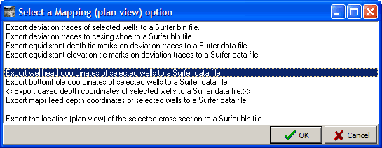
Click Export wellhead coordinates ... and click OK.
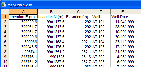
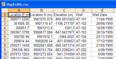
The result is a csv file: select a folder and file name and click OK. Here is part of the file, opened in a spreadsheet:
Use the wells already tagged. Click Map again:
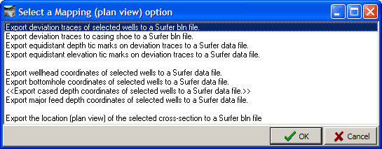
Click Export deviation traces ... and click OK.
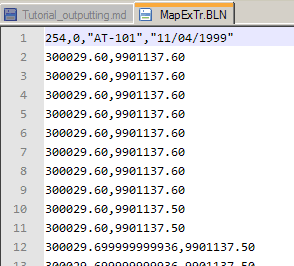
The result is a bln file: select a folder and file name and click OK. Here is part of the file, opened in a text editor:
Use the wells already tagged. Click Map again:
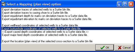
Click Export bottomhole coordinates ... and click OK.
The result is a csv file: select a folder and file name and click OK. Here is part of the file, opened in a spreadsheet:
Start Surfer. This assumes you know how to use Surfer.
Import the geo-referenced topographical map as a base layer.
Import the file of wellhead coordinates as a post layer. Call it Wellheads. Assign each wellhead a small blue star.
Import the file of bottomhole coordinates as a post layer. Call it Wellbases. Label each wellbase with the well name, just above the bottom of the well.
Import the file of well traces as a base layer. Call it Well traces.
Import the file of temperature at -500 m elevation as a post layer. Call this Temp@-500m. Assign each location (where the well trace is at -500 m elevation) a red dot.
Invoke Data: Grid to convert the file of temperature at -500 m elevation to a contour. Call this Temp@-500m as well.
Create and place a color scale for the contour just right of the contour.
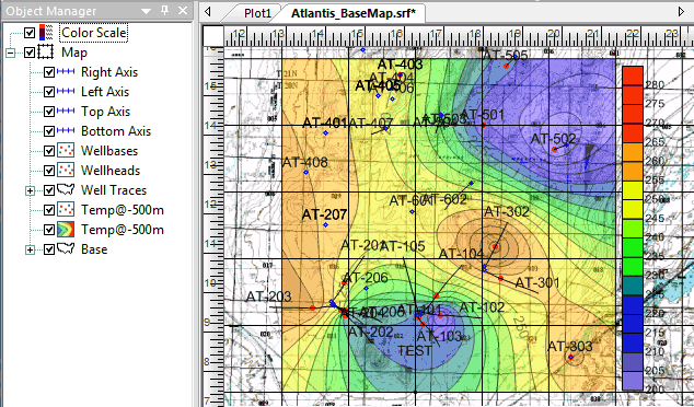
Voila:
In part 1 of this tutorial, you selected wells to display on the Surfer map at the node Well and Drilling: Location and Deviation. However, you can choose wells at any other node that displays wells. For example, to display on the Surfer map only wells with STATIC interpreted temperatures, first tag these data sets:
Go to the node Interpreted: Temperature.
In the filter bar, click and click Default Filter in case the filter was different.
Select temperature data sets of type STATIC: In the filter bar, click the to the right of Reference ID and click STATIC in the list. Click Tag All:
Those steps are the same as in part 4 of this tutorial, above. Now, create the three files of wellhead coordinates, well traces and bottomhole coordinates. For each file:
Click Map
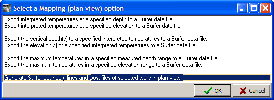
Click Generate Surfer boundary lines and post files ... and click OK.
Proceed as you did above to create these three files.