Introduction
Tutorials
Improving a discharge simulation
An injection simulation is the calculated pressure and temperature down a well injection at a steady-state mass flowrate read more.
An injection simulation can be TopDown or a BottomUp. This describes a TopDown simulation.
This tutorial uses:
data from the measured injectivity curve Test rate data - 1 that you should have entered earlier.
the measured injection profile 860 t/hr that you should have entered earlier.
Entering and running an injection simulation is similar to a discharge simulation. If you are unsure what to do here, review discharge simulations.
This tutorial covers pumped injection wells, where for all mass flowrates the fluid has to be pumped into the well, the wellhead pressure is positive and the fluid is liquid throughout the well. For these wells, the Start depth is always zero.
Free-flowing wells can (perhaps only at low mass flowrates) accept fluid without pumping and have a wellhead pressure close to zero, see this tutorial. For these wells, Start depth will be greater than zero.
This tutorial uses one set of wellhead measurements from the measured injectivity curve Test rate data - 1: 860 t/hr, 110 barg, 50 degrees C:
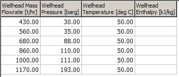
Also assume CO2 is 5,000 ppm and NaCl is 0 ppm (in total fluid).
In the sample database, open a new injection simulation for  .
.
Enter the data assumed above:
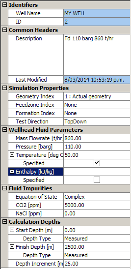
Note: - Measure all depths relative to the same point at the wellhead read more. - Ensure there is a tick under Temperature and no tick under Enthalpy.
Run and save the injection simulation. If you get the error Solution did not converge see here.
Display a Quick Graph of the new injection simulation:
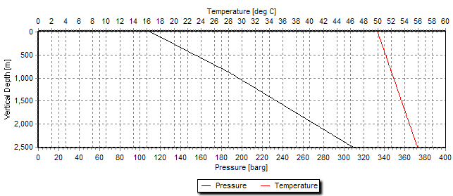
I changed the graph to look like this.
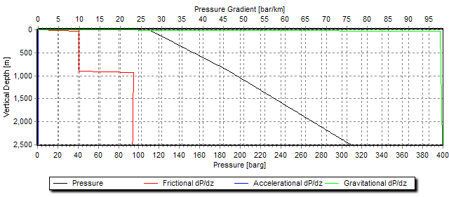
The discontinuity in pressure is caused by an increase in friction (red series) below 900 m, where the casing changes to slotted liner.
The pressure loss due to friction is about 1 km of 10 barg/km and 1.5 km of 23 barg/km: about 45 barg total.
The gravitational change in pressure is simply the static pressure of water in the well at that depth, about 2.5 km of about 100 barg/km; about 250 barg total.
The expected pressure difference between the wellhead is thus 250 barg less the 45 barg of friction, about 205 barg. This is about the difference shown on the graph above.
Click the  tab.
tab.
From the Measured profile dropdown list, select 860t/hr that you created earlier. Tick Visible to see the measured and calculated profile.
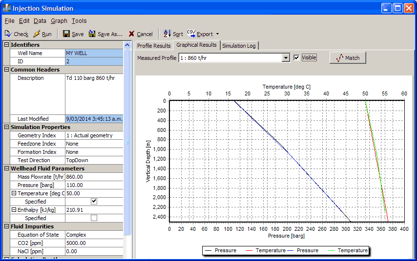
If your graph does not look like this, change it. To see the difference between the measured and calculated profile you need to turn Show points off, which hides the fact that the measured profile only has three points.
The calculated (black and red series) and measured (blue and green series) profiles match well.
Click Match to compare them.
You can now try to improve the injection simulation by changing the assumed data, as you did for a discharge simulation. For example, change the impurity concentrations read how. Unlike for a discharge simulation, fluid loss at a secondary loss zone only slightly affects the downhole injection pressure and temperature profiles, so you can't find secondary feedzones this way.